Artificial intelligence, machine learning, and computer vision are fields too broad to be even introduced in this Supplementary Methods section. That is why we focus on briefly introducing the basic concepts on neural networks, convolutional neural networks, transfer learning, data augmentation, and visualization techniques like gradient-weighted class activation maps and saliency maps, which are the most relevant topics for this manuscript. We provide selected citations so that the interested reader can start exploring these topics in more depth. Other concepts such as optimizers, minibatch gradient descent, vanishing gradients, exploding gradients, batch normalization, and dropout layers are not as crucial to understand this manuscript and are, therefore, left for the interested reader to explore.
Neural Networks 
Neural networks are complex mathematical functions that map input(s) (for example, MRI image(s)) to output(s) (for example, label(s) like "tubers" or "no tubers"). Although neural networks can have extremely complex architectures with millions of parameters, an initial approach to understand them is to think of them as a combination of relatively simple methods such as the perceptron. Excellent explanations of the perceptron can be found at: https://blog.knoldus.com/introduction-to-perceptron-neural-network/, https://towardsdatascience.com/what-the-hell-is-perceptron-626217814f53, and https://www.toptal.com/machine-learning/an-introduction-to-deep-learning-from-perceptrons-to-deep-networks.
One of the major strengths of neural networks is that they combine several layers of relatively simple methods (for example, the perceptron) to build extremely complex classifiers. An excellent and very clear introductory academic article to neural networks is LeCun Y, Bengio Y, Hinton G. Deep learning. Nature. 2015 May 28;521(7553):436-44. doi: 10.1038/nature14539 at: https://www.ncbi.nlm.nih.gov/pubmed/26017442. Neural networks try to classify the input(s) as belonging to one of a series of classes (we will ignore neural networks that predict a continuous outcome as they are not relevant for this manuscript).
Neural networks learn iteratively. During training, the initial weights in a neural network are random (unless transfer learning is used, as explained below). Therefore, when the class of the initial input(s) is predicted, the output(s) is(are) a random guess. However, this initial random guess is very informative. The real classification of the input(s) (label) is compared with the generated output(s) via a proper loss function. The loss function is a mathematical quantification of how far away the predicted output(s) is from the real classification (the label). For binary classification tasks, as in this manuscript, a common option is the binary cross-entropy loss. The goal during training is to minimize the loss function. For this, the error in classification (how far the predicted output(s) is from the real classification) is backpropagated to the weights in the neural network.
Backpropagation is a key feature that allow neural networks to learn. Using partial derivatives, backpropagation breaks down the classification error into its components, each of which is attributable to each weight. Intuitively, it quantitifies how much each weight contributed to the final error. Backpropagation also modifies each weight a small amount in the direction to minimize its error. Therefore, by modifying each weight in the direction of decreasing the error the total error is expected to be reduced and the loss function is expected to decrease with this initial backpropagation step. After this initial backpropagation step, the neural network does not have entirely random weights, but weights that have been slightly tuned to improve prediction. At this point the neural network is presented with a second input(s). A predicted outcome is computed in a new forward pass and then the predicted classification is compared with the real classification of the input(s). The error is calculated again with the loss function and the errors are backpropagated so that the weights are slightly tuned to further reduce error.
This iterative process of:
Computing predictions with a forward pass.
Quantifying the error with the loss function.
Backpropagating the error and tuning the weights to reduce errors.
is repeated multiple times to make the neural networks learn the relationship between the input and the classes.
Excellent explanations of these concepts can be found at: https://medium.com/datathings/neural-networks-and-backpropagation-explained-in-a-simple-way-f540a3611f5e and https://becominghuman.ai/basics-of-neural-network-bef2ba97d2cf.
A (highly recommended) simple interactive neural network that the reader can train and helps solidify these concepts can be found at: https://playground.tensorflow.org/.
Convolutional Neural Networks 
An excellent and very clear introductory academic article to convolutional neural networks is LeCun Y, Bengio Y, Hinton G. Deep learning. Nature. 2015 May 28;521(7553):436-44. doi: 10.1038/nature14539 at: https://www.ncbi.nlm.nih.gov/pubmed/26017442.
Most machine learning methods need the raw input features to be preprocessed by a human to transform them into features that the method can work with. This task, termed "feature engineering" requires vast amount of human effort and domain knowledge. One of the major advantages of neural networks is that the relevant information from the raw data is extracted automatically as long as a large enough number of examples for each class is presented to the neural network.
Different types of raw features are preprocessed differently. Convolutional neural networks process the features taking advantage of information present in the structure of the data. In an image classification task, like the one in this manuscript, the spatial relationship between the pixels is a relevant structure that the neural network can take advantage of because pixels that are close to each other are more likely to be similar than pixels that are far from each other. The detection of areas of the image where pixels vary abruptly is also a structure the neural network can take advantage of because they may represent edges: limits between different objects in the image.
Convolutional layers in the neural network can be loosely thought of as filters that "feature engineer" the raw image to extract relevant information such as edges or basic shapes. Using pooling layers, the most relevant basic features are kept while the non-informative portions of the image are discarded in a progressive reduction of the image. Several combinations of convolutional layers followed by pooling layers achieve extraction of relevant features that are increasingly more abstract as the neural networks become deeper. Excellent and visual explanations of convolutional and pooling layers can be found at: https://towardsdatascience.com/intuitively-understanding-convolutions-for-deep-learning-1f6f42faee1, https://devblogs.nvidia.com/deep-learning-nutshell-core-concepts/ and https://medium.com/technologymadeeasy/the-best-explanation-of-convolutional-neural-networks-on-the-internet-fbb8b1ad5df8.
The final layers of a convolutional neural network are "dense" or "fully-connected" layers (they can be loosely thought of as layers of perceptrons) that classify the input based on the relevant features already "feature engineered" by the previous layers of the network.
A (highly recommended) excellent interactive visualization of a convolutional neural network that the reader can use and helps solidify these concepts can be found at: http://scs.ryerson.ca/~aharley/vis/conv/.
Types of convolutional neural network architectures
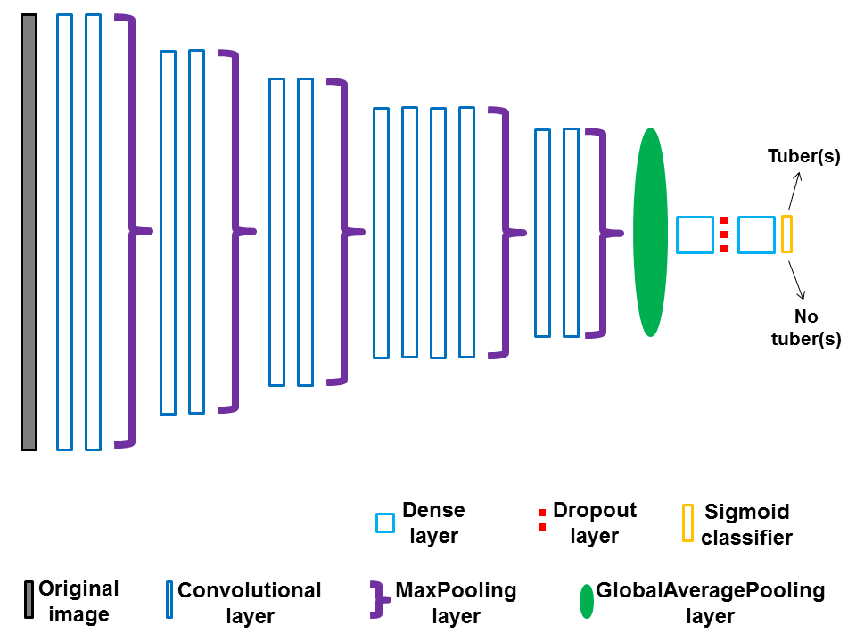
Our custom created TSCCNN convolutional neural network has an architecture where learning occurs stepwise: each block of convolutional and pooling layers extracts progressively more abstract information until the final fully connected layers classify the images into a class.
TSCCNN architecture:
More recent architectures refine this approach in two different ways (the explanations and references for these approaches are necessarily more technical, although we hope to provide an intuitive global idea):
Split-transform-merge architectures that allow deeper and wider convolutional neural networks while keeping computations efficient and avoiding overfitting. The InceptionV3 used in this manuscript is a common example of this family of architectures. Excellent academic articles can be found at: https://arxiv.org/pdf/1409.4842.pdf and https://arxiv.org/pdf/1512.00567.pdf. Excellent explanations of this approach can be found at: https://towardsdatascience.com/a-simple-guide-to-the-versions-of-the-inception-network-7fc52b863202 and https://www.analyticsvidhya.com/blog/2018/10/understanding-inception-network-from-scratch/.
Residual network architectures that can be understood as ensembles of multiple relatively shallow classifiers that, when combined, become a very good classifier. Another intuitive approach to understand residual architectures is that each shallow classifier focuses especially on the errors of the other shallow classifiers, so that each shallow classifier "learns what was not learned by the other classifiers" and then the results are combined. The ResNet50 used in this manuscript is a common example of this family of architectures. Excellent academic articles can be found at: https://arxiv.org/pdf/1605.06431.pdf, https://www.aimspress.com/article/10.3934/mbe.2019165/fulltext.html (Figure 4 in that article shows the CNN architecture), and https://arxiv.org/pdf/1611.05431.pdf. Excellent explanations of this approach can be found at: https://towardsdatascience.com/an-overview-of-resnet-and-its-variants-5281e2f56035 and https://cv-tricks.com/cnn/understand-resnet-alexnet-vgg-inception/.
Transfer Learning 
The concept of transfer learning is relatively easy to grasp. Initializing neural networks with random weights requires multiple steps of forward pass and backpropagation to finely tune the weights to learn the specific task that is being learned. Transfer learning uses the weights of a neural network already trained in a similar task as initial weights to be tuned. For example, in this manuscript, we used the the ImageNet weights for InceptionV3 and ResNet50. The ImageNet weights are the optimal weights for classifying images into classes such as cat, dog, ship, building, etc. in the ImageNet competition. It does not appear intuitive that these weights may be helpful to classify MRI images with and without tubers. However, it is important to remember that a major part of the weights within a convolutional neural network learn essential features such as edges and their combinations into basic shapes. These weights are more easily finely tuned to the specific task than random initial weights that have to be trained to recognize edges and basic shapes in the first place. As an illustration, in this article, InceptionV3 and ResNet50 convolutional neural networks initialized with the ImageNet weights trained much faster and performed much better in the validation set than the TSCCNN convolutional neural network, which was initialized with random weights.
An excellent academic article on transfer learning can be found at: https://arxiv.org/pdf/1808.01974.pdf. Excellent explanations of transfer learning can be found at: https://machinelearningmastery.com/transfer-learning-for-deep-learning/ and https://medium.com/kansas-city-machine-learning-artificial-intelligen/an-introduction-to-transfer-learning-in-machine-learning-7efd104b6026.
Minimizing overfitting 
Convolutional neural networks are complex mathematical functions with a huge number of parameters, which allows them to fit well complex datasets but, at the same time, makes them prone to fit the data too well: overfitting. Overfitting occurs when the model recognizes some patterns in the data, but these patterns exist only in the specific dataset and are not generalizable.
There are several ways to minimize overfitting, some common to all convolutional neural networks and some more specific to situations where there is a relatively small number of training examples.
Among the general methods to minimize overfitting in convolutional neural networks, the most commonly used and powerful one is to completely separate training, validation, and test sets. With this method generalizability is evaluated because the convolutional neural network ability to detect patterns is tested in data it never saw before: the test set. Explanations of the rationale for training, validation, and test sets can be found here https://deeplizard.com/learn/video/Zi-0rlM4RDs and here https://towardsdatascience.com/train-validation-and-test-sets-72cb40cba9e7.
Other general methods to minimize overfitting in convolutional neural networks consist of avoiding the convolutional neural network to fit too well the training dataset. These include addition of random noise, batch normalization, dropout, and global average pooling. The global idea behind all these methods is making the training data “fuzzier” (note that this is a simplification of reality, the methods are more complicated) so that the convolutional neuronal is able to fit the features that are most characteristic of the pattern of interest, but not the noise that randomly appears in the training dataset and is not generalizable to other datasets. Explanations of these methods can be found here https://machinelearningmastery.com/train-neural-networks-with-noise-to-reduce-overfitting/, https://towardsdatascience.com/batch-normalization-in-neural-networks-1ac91516821c, https://machinelearningmastery.com/dropout-for-regularizing-deep-neural-networks/, and here https://alexisbcook.github.io/2017/global-average-pooling-layers-for-object-localization/.
Finally, a method that is typically used when the number of training examples is relatively small is data augmentation. Data augmentation, explained below, regularizes and makes convolutional neural networks more robust to noise.
Data Augmentation 
Convolutional neural networks need large amounts of labelled data because no explicit programming is provided for their learning. They have to learn by example, so they need multiple examples. When datasets are not as large as desired a solution is to expand existing data in the training set with artificial examples created synthetically.
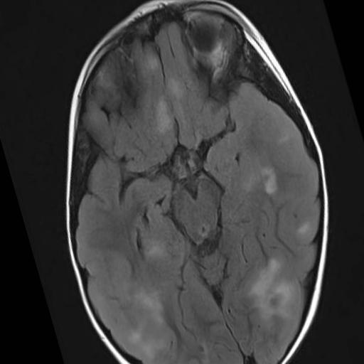
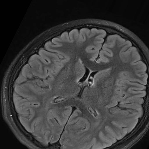
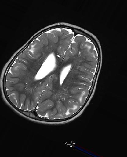
For example, in our manuscript, we created approximately 4 images per original image by allowing random rotation, shift, horizontal flip, and zoom of the original images. Data augmentation does not only provide more examples for learning. It is also a form of regularization: that is, the convolutional neural network becomes more resistant to noisy features such as size or location of the pattern within the image and more robust to the main features that define that particular pattern (tuber in the case of this manuscript).
The image on the left (TSC patient) has been rotated and zoomed in. The center image (Control) has been rotated and zoomed in even more. The image on the right (TSC patient) has been rotated, shifted, zoomed out, and flipped (pay attention at the reversed letters in the lower right corner).
 |
 |
 |
An excellent academic article on data augmentation can be found at: https://arxiv.org/pdf/1712.04621.pdf. Excellent explanations on data augmentation can be found at: https://medium.com/nanonets/how-to-use-deep-learning-when-you-have-limited-data-part-2-data-augmentation-c26971dc8ced and https://towardsdatascience.com/data-augmentation-and-images-7aca9bd0dbe8.